Batch normalization, as described in the March 2015 paper (the BN2015 paper) by Sergey Ioffe and Christian Szegedy, is a simple and effective way to improve the performance of a neural network. In the BN2015 paper, Ioffe and Szegedy show that batch normalization enables the use of higher learning rates, acts as a regularizer and can speed up training by 14 times. In this post, I show how to implement batch normalization in Tensorflow.
Edit 2018 (that should have been made back in 2016): If you’re just looking for a working implementation, Tensorflow has an easy to use batch_normalization layer in the tf.layers module. Just be sure to wrap your training step in a with tf.control_dependencies(tf.get_collection(tf.GraphKeys.UPDATE_OPS)): and it will work.
Edit 07/12/16: I’ve updated this post to cover the calculation of population mean and variance at test time in more detail.
Edit 02/08/16: In case you are looking for recurrent batch normalization (i.e., from Cooijmans et al. (2016)), I have uploaded a working Tensorflow implementation here. The only tricky part of the implementation, as compared to the feedforward batch normalization presented this post, is storing separate population variables for different timesteps.
The problem
Batch normalization is intended to solve the following problem: Changes in model parameters during learning change the distributions of the outputs of each hidden layer. This means that later layers need to adapt to these (often noisy) changes during training.
Batch normalization in brief
To solve this problem, the BN2015 paper propposes the batch normalization of the input to the activation function of each nuron (e.g., each sigmoid or ReLU function) during training, so that the input to the activation function across each training batch has a mean of 0 and a variance of 1. For example, applying batch normalization to the activation would result in where is the batch normalizing transform.
The batch normalizing transform
To normalize a value across a batch (i.e., to batch normalize the value), we subtract the batch mean, , and divide the result by the batch standard deviation, . Note that a small constant is added to the variance in order to avoid dividing by zero.
Thus, the initial batch normalizing transform of a given value, , is:
Because the batch normalizing transform given above restricts the inputs to the activation function to a prescribed normal distribution, this can limit the representational power of the layer. Therefore, we allow the network to undo the batch normalizing transform by multiplying by a new scale parameter and adding a new shift parameter . and are learnable parameters.
Adding in and producing the following final batch normalizing transform:
Implementing batch normalization in Tensorflow
We will add batch normalization to a basic fully-connected neural network that has two hidden layers of 100 neurons each and show a similar result to Figure 1 (b) and (c) of the BN2015 paper.
Note that this network is not yet generally suitable for use at test time. See the section Making predictions with the model below for the reason why, as well as a fixed version.
Imports, config
import numpy as np, tensorflow as tf, tqdm
from tensorflow.examples.tutorials.mnist import input_data
import matplotlib.pyplot as plt
%matplotlib inline
mnist = input_data.read_data_sets('MNIST_data', one_hot=True)
# Generate predetermined random weights so the networks are similarly initialized
w1_initial = np.random.normal(size=(784,100)).astype(np.float32)
w2_initial = np.random.normal(size=(100,100)).astype(np.float32)
w3_initial = np.random.normal(size=(100,10)).astype(np.float32)
# Small epsilon value for the BN transform
epsilon = 1e-3Building the graph
# Placeholders
x = tf.placeholder(tf.float32, shape=[None, 784])
y_ = tf.placeholder(tf.float32, shape=[None, 10])
# Layer 1 without BN
w1 = tf.Variable(w1_initial)
b1 = tf.Variable(tf.zeros([100]))
z1 = tf.matmul(x,w1)+b1
l1 = tf.nn.sigmoid(z1)Here is the same layer 1 with batch normalization:
# Layer 1 with BN
w1_BN = tf.Variable(w1_initial)

# Note that pre-batch normalization bias is ommitted. The effect of this bias would be
# eliminated when subtracting the batch mean. Instead, the role of the bias is performed
# by the new beta variable. See Section 3.2 of the BN2015 paper.
z1_BN = tf.matmul(x,w1_BN)

# Calculate batch mean and variance
batch_mean1, batch_var1 = tf.nn.moments(z1_BN,[0])

# Apply the initial batch normalizing transform
z1_hat = (z1_BN - batch_mean1) / tf.sqrt(batch_var1 + epsilon)

# Create two new parameters, scale and beta (shift)
scale1 = tf.Variable(tf.ones([100]))
beta1 = tf.Variable(tf.zeros([100]))

# Scale and shift to obtain the final output of the batch normalization
# this value is fed into the activation function (here a sigmoid)
BN1 = scale1 * z1_hat + beta1
l1_BN = tf.nn.sigmoid(BN1)
# Layer 2 without BN
w2 = tf.Variable(w2_initial)
b2 = tf.Variable(tf.zeros([100]))
z2 = tf.matmul(l1,w2)+b2
l2 = tf.nn.sigmoid(z2)Note that tensorflow provides a tf.nn.batch_normalization, which I apply to layer 2 below. This code does the same thing as the code for layer 1 above. See the documentation here and the code here.
# Layer 2 with BN, using Tensorflows built-in BN function
w2_BN = tf.Variable(w2_initial)
z2_BN = tf.matmul(l1_BN,w2_BN)
batch_mean2, batch_var2 = tf.nn.moments(z2_BN,[0])
scale2 = tf.Variable(tf.ones([100]))
beta2 = tf.Variable(tf.zeros([100]))
BN2 = tf.nn.batch_normalization(z2_BN,batch_mean2,batch_var2,beta2,scale2,epsilon)
l2_BN = tf.nn.sigmoid(BN2)
# Softmax
w3 = tf.Variable(w3_initial)
b3 = tf.Variable(tf.zeros([10]))
y = tf.nn.softmax(tf.matmul(l2,w3)+b3)
w3_BN = tf.Variable(w3_initial)
b3_BN = tf.Variable(tf.zeros([10]))
y_BN = tf.nn.softmax(tf.matmul(l2_BN,w3_BN)+b3_BN)# Loss, optimizer and predictions
cross_entropy = -tf.reduce_sum(y_*tf.log(y))
cross_entropy_BN = -tf.reduce_sum(y_*tf.log(y_BN))
train_step = tf.train.GradientDescentOptimizer(0.01).minimize(cross_entropy)
train_step_BN = tf.train.GradientDescentOptimizer(0.01).minimize(cross_entropy_BN)
correct_prediction = tf.equal(tf.arg_max(y,1),tf.arg_max(y_,1))
accuracy = tf.reduce_mean(tf.cast(correct_prediction,tf.float32))
correct_prediction_BN = tf.equal(tf.arg_max(y_BN,1),tf.arg_max(y_,1))
accuracy_BN = tf.reduce_mean(tf.cast(correct_prediction_BN,tf.float32))Training the network
zs, BNs, acc, acc_BN = [], [], [], []

sess = tf.InteractiveSession()
sess.run(tf.global_variables_initializer())
for i in tqdm.tqdm(range(40000)):
    batch = mnist.train.next_batch(60)
    train_step.run(feed_dict={x: batch[0], y_: batch[1]})
    train_step_BN.run(feed_dict={x: batch[0], y_: batch[1]})
    if i % 50 is 0:
        res = sess.run([accuracy,accuracy_BN,z2,BN2],feed_dict={x: mnist.test.images, y_: mnist.test.labels})
        acc.append(res[0])
        acc_BN.append(res[1])
        zs.append(np.mean(res[2],axis=0)) # record the mean value of z2 over the entire test set
        BNs.append(np.mean(res[3],axis=0)) # record the mean value of BN2 over the entire test set

zs, BNs, acc, acc_BN = np.array(zs), np.array(BNs), np.array(acc), np.array(acc_BN)
Improvements in speed and accuracy
As seen below, there is a noticeable improvement in the accuracy and speed of training. As shown in figure 2 of the BN2015 paper, this difference can be very significant for other network architectures.
fig, ax = plt.subplots()

ax.plot(range(0,len(acc)*50,50),acc, label='Without BN')
ax.plot(range(0,len(acc)*50,50),acc_BN, label='With BN')
ax.set_xlabel('Training steps')
ax.set_ylabel('Accuracy')
ax.set_ylim([0.8,1])
ax.set_title('Batch Normalization Accuracy')
ax.legend(loc=4)
plt.show()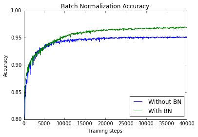
Illustration of input to activation functions over time
Below is the distribution over time of the inputs to the sigmoid activation function of the first five neurons in the network’s second layer. Batch normalization has a visible and significant effect of removing variance/noise in these inputs. As described by Ioffe and Szegedy, this allows the third layer to learn faster and is responsible for the increase in accuracy and learning speed. See Figure 1 and Section 4.1 of the BN2015 paper.
fig, axes = plt.subplots(5, 2, figsize=(6,12))
fig.tight_layout()

for i, ax in enumerate(axes):
    ax[0].set_title("Without BN")
    ax[1].set_title("With BN")
    ax[0].plot(zs[:,i])
    ax[1].plot(BNs[:,i])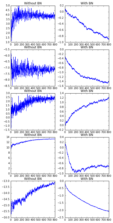
Making predictions with the model
When using a batch normalized model at test time to make predictions, using the batch mean and batch variance can be counter-productive. To see this, consider what happens if we feed a single example into the trained model above: the inputs to our activation functions will always be 0 (since we are normalizing them to have a mean of 0), and we will always get the same prediction, regardless of the input!
To demonstrate:
predictions = []
correct = 0
for i in range(100):
    pred, corr = sess.run([tf.arg_max(y_BN,1), accuracy_BN],
                         feed_dict={x: [mnist.test.images[i]], y_: [mnist.test.labels[i]]})
    correct += corr
    predictions.append(pred[0])
print("PREDICTIONS:", predictions)
print("ACCURACY:", correct/100)
PREDICTIONS: [8, 8, 8, 8, 8, 8, 8, 8, 8, 8, 8, 8, 8, 8, 8, 8, 8, 8, 8, 8, 8, 8, 8, 8, 8, 8, 8, 8, 8, 8, 8, 8, 8, 8, 8, 8, 8, 8, 8, 8, 8, 8, 8, 8, 8, 8, 8, 8, 8, 8, 8, 8, 8, 8, 8, 8, 8, 8, 8, 8, 8, 8, 8, 8, 8, 8, 8, 8, 8, 8, 8, 8, 8, 8, 8, 8, 8, 8, 8, 8, 8, 8, 8, 8, 8, 8, 8, 8, 8, 8, 8, 8, 8, 8, 8, 8, 8, 8, 8, 8]
ACCURACY: 0.02Our model always predicts 8, and there appear to be only two 8s in the first 100 MNIST test samples, for an accuracy of 2%.
Fixing the model for test time
To fix this, we need to replace the batch mean and batch variance in each batch normalization step with estimates of the population mean and population variance, respectively. See Section 3.1 of the BN2015 paper. Testing the model above only worked because the entire test set was predicted at once, so the “batch mean” and “batch variance” of the test set provided good estimates for the population mean and population variance.
To make a batch normalized model generally suitable for testing, we want to obtain estimates for the population mean and population variance at each batch normalization step before test time (i.e., during training), and use these values when making predictions. Note that for the same reason that we need batch normalization (i.e. the mean and variance of the activation inputs changes during training), it would be best to estimate the population mean and variance after the weights they depend on are trained, although doing these simultaneously is not the worst offense, since the weights are expected to converge near the end of training.
And now, to actually implement this in Tensorflow, we will write a batch_norm_wrapper function, which we will use to wrap the inputs to our activation functions. The function will store the population mean and variance as tf.Variables, and decide whether to use the batch statistics or the population statistics for normalization. To do this, it makes use of an is_training flag. Because we need to learn the population mean and variance during training, we do this when is_training == True. Here is an outline of the code:
def batch_norm_wrapper(inputs, is_training):
    ...
    pop_mean = tf.Variable(tf.zeros([inputs.get_shape()[-1]]), trainable=False)
    pop_var = tf.Variable(tf.ones([inputs.get_shape()[-1]]), trainable=False)

    if is_training:
        mean, var = tf.nn.moments(inputs,[0])
        ...
        # learn pop_mean and pop_var here
        ...
        return tf.nn.batch_normalization(inputs, batch_mean, batch_var, beta, scale, epsilon)
    else:
        return tf.nn.batch_normalization(inputs, pop_mean, pop_var, beta, scale, epsilon)
Note that the variables have been declared with a trainable = False argument, since we will be updating these ourselves rather than having the optimizer do it.
One approach to estimating the population mean and variance during training is to use an exponential moving average, though strictly speaking, a simple average over the sample would be (marginally) better. The exponential moving average is simple and lets us avoid extra work, so we use that:
decay = 0.999 # use numbers closer to 1 if you have more data
train_mean = tf.assign(pop_mean, pop_mean * decay + batch_mean * (1 - decay))
train_var = tf.assign(pop_var, pop_var * decay + batch_var * (1 - decay))
Finally, we will need a way to call these training ops. For full control, you can add them to a graph collection (see the link to Tensorflow’s code below), but for simplicity, we will call them every time we calculate the batch_mean and batch_var. To do this, we add them as dependencies to the return value of batch_norm_wrapper when is_training is true. Here is the final batch_norm_wrapper function:
# this is a simpler version of Tensorflow's 'official' version. See:
# https://github.com/tensorflow/tensorflow/blob/master/tensorflow/contrib/layers/python/layers/layers.py#L102
def batch_norm_wrapper(inputs, is_training, decay = 0.999):

    scale = tf.Variable(tf.ones([inputs.get_shape()[-1]]))
    beta = tf.Variable(tf.zeros([inputs.get_shape()[-1]]))
    pop_mean = tf.Variable(tf.zeros([inputs.get_shape()[-1]]), trainable=False)
    pop_var = tf.Variable(tf.ones([inputs.get_shape()[-1]]), trainable=False)

    if is_training:
        batch_mean, batch_var = tf.nn.moments(inputs,[0])
        train_mean = tf.assign(pop_mean,
                               pop_mean * decay + batch_mean * (1 - decay))
        train_var = tf.assign(pop_var,
                              pop_var * decay + batch_var * (1 - decay))
        with tf.control_dependencies([train_mean, train_var]):
            return tf.nn.batch_normalization(inputs,
                batch_mean, batch_var, beta, scale, epsilon)
    else:
        return tf.nn.batch_normalization(inputs,
            pop_mean, pop_var, beta, scale, epsilon)
An implementation that works at test time
And now to demonstrate that this works, we rebuild/retrain the model with our batch_norm_wrapper function. Note that we need to build the graph once for training, and then again at test time, so we write a build_graph function (in practice, this would usually be encapsulated in a model object):
def build_graph(is_training):
    # Placeholders
    x = tf.placeholder(tf.float32, shape=[None, 784])
    y_ = tf.placeholder(tf.float32, shape=[None, 10])

    # Layer 1
    w1 = tf.Variable(w1_initial)
    z1 = tf.matmul(x,w1)
    bn1 = batch_norm_wrapper(z1, is_training)
    l1 = tf.nn.sigmoid(bn1)

    #Layer 2
    w2 = tf.Variable(w2_initial)
    z2 = tf.matmul(l1,w2)
    bn2 = batch_norm_wrapper(z2, is_training)
    l2 = tf.nn.sigmoid(bn2)

    # Softmax
    w3 = tf.Variable(w3_initial)
    b3 = tf.Variable(tf.zeros([10]))
    y  = tf.nn.softmax(tf.matmul(l2, w3))

    # Loss, Optimizer and Predictions
    cross_entropy = -tf.reduce_sum(y_*tf.log(y))

    train_step = tf.train.GradientDescentOptimizer(0.01).minimize(cross_entropy)

    correct_prediction = tf.equal(tf.arg_max(y,1),tf.arg_max(y_,1))
    accuracy = tf.reduce_mean(tf.cast(correct_prediction,tf.float32))

    return (x, y_), train_step, accuracy, y, tf.train.Saver()
#Build training graph, train and save the trained model
sess.close()
tf.reset_default_graph()
(x, y_), train_step, accuracy, _, saver = build_graph(is_training=True)
acc = []
with tf.Session() as sess:
sess.run(tf.global_variables_initializer())
for i in tqdm.tqdm(range(10000)):
batch = mnist.train.next_batch(60)
train_step.run(feed_dict={x: batch[0], y_: batch[1]})
if i % 50 is 0:
res = sess.run([accuracy],feed_dict={x: mnist.test.images, y_: mnist.test.labels})
acc.append(res[0])
saved_model = saver.save(sess, './temp-bn-save')
print("Final accuracy:", acc[-1])Final accuracy: 0.9721And now to show that this worked, we repeat our experiment of predicting examples one by one:
tf.reset_default_graph()
(x, y_), _, accuracy, y, saver = build_graph(is_training=False)

predictions = []
correct = 0
with tf.Session() as sess:
    sess.run(tf.global_variables_initializer())
    saver.restore(sess, './temp-bn-save')
    for i in range(100):
        pred, corr = sess.run([tf.arg_max(y,1), accuracy],
                             feed_dict={x: [mnist.test.images[i]], y_: [mnist.test.labels[i]]})
        correct += corr
        predictions.append(pred[0])
print("PREDICTIONS:", predictions)
print("ACCURACY:", correct/100)
PREDICTIONS: [7, 2, 1, 0, 4, 1, 4, 9, 6, 9, 0, 6, 9, 0, 1, 5, 9, 7, 3, 4, 9, 6, 6, 5, 4, 0, 7, 4, 0, 1, 3, 1, 3, 4, 7, 2, 7, 1, 2, 1, 1, 7, 4, 2, 3, 5, 1, 2, 4, 4, 6, 3, 5, 5, 6, 0, 4, 1, 9, 5, 7, 8, 9, 3, 7, 4, 6, 4, 3, 0, 7, 0, 2, 9, 1, 7, 3, 2, 9, 7, 7, 6, 2, 7, 8, 4, 7, 3, 6, 1, 3, 6, 9, 3, 1, 4, 1, 7, 6, 9]
ACCURACY: 0.99