The unit circle: everybody’s favorite circle.
I recently needed to an annotated unit circle for some teaching material I was preparing. Rather than using one of the countless pictures already available, I thought it was a good excuse to play around a bit with using mathematical annotations in ggplot2. This post explains the process.
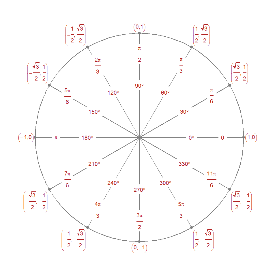
Here’s what we’ll be working towards:
We start by defining a function that, given a radius, generates a data frame of coordinates of a circle centered around the origin.
library(tidyverse)
library(scales)
library(stringr)

get_circle_coords <- function(r = 1, ...) {
  data_frame(theta = seq(0, 2 * pi, ...),
             x     = cos(theta) * r,
             y     = sin(theta) * r)
}

circ <- get_circle_coords(length.out = 200)
qplot(circ$x, circ$y, geom = "path")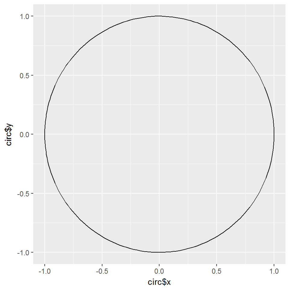
Next, we want to generate the coordinates where we go around the unit circle by one-sixth \(\pi\) at each step (we drop the last observation to avoid overlap):
coords_pi <- get_circle_coords(by = pi / 6) %>% head(-1)We can now plot the circle itself as a geom_path, the hubs as geom_point, and spokes as geom_segment. theme_void drops all unnecessary chart junk, and coord_equal makes sure that one unit on the x-axis is equivalent to one unit on the y-axis.
ggplot(coords_pi, aes(x = x, y = y)) +
  geom_path(data = circ, color = "grey50") +
  geom_point(color = "grey50") +
  geom_segment(aes(xend = 0, yend = 0), color = "grey50") +
  xlim(-1.2, 1.2) +
  ylim(-1.2, 1.2) +
  theme_void() +
  coord_equal()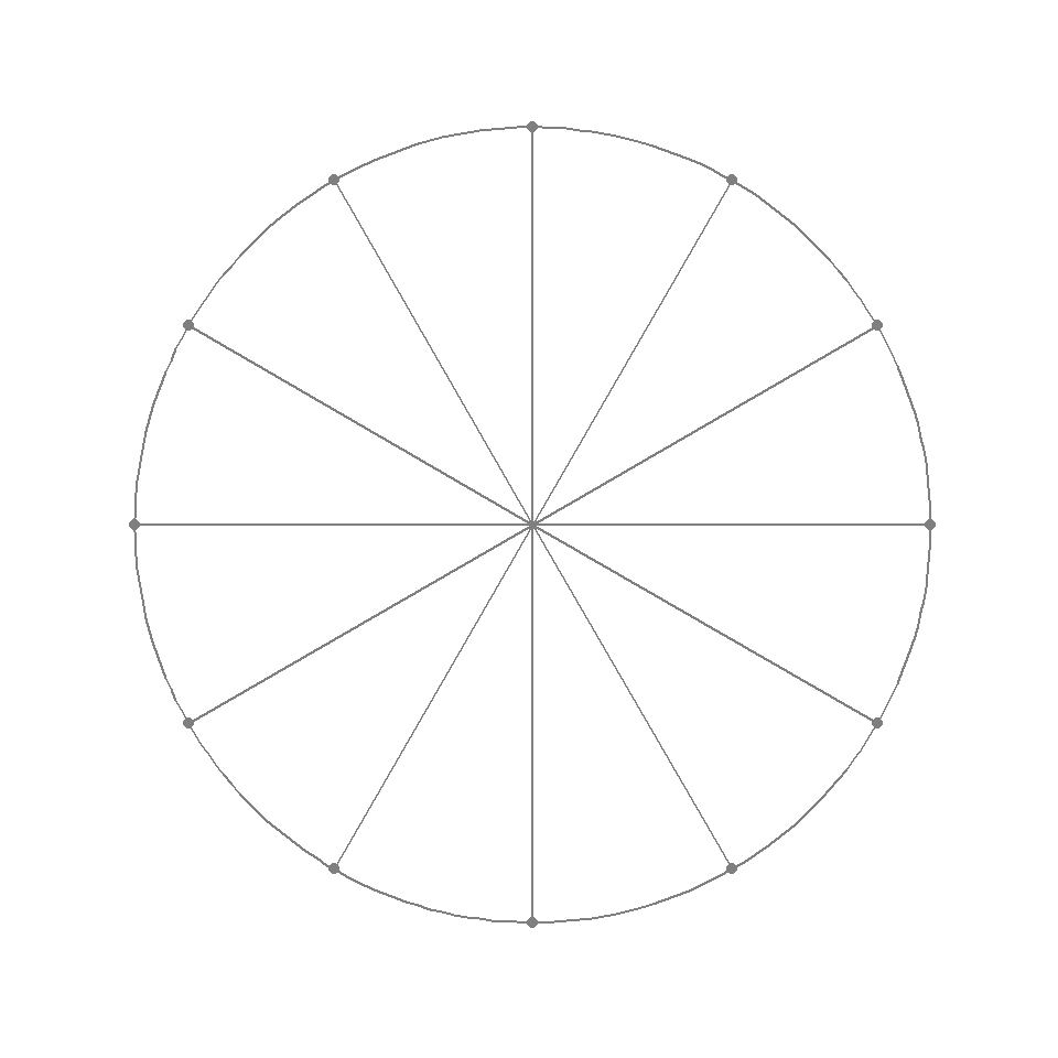
We add a character variable that gives the equivalent angles in degrees:
coords_pi$angle <- seq(0, 330, 30) %>% paste(" * degree")To properly typeset the fractions of \(\pi\) we use R’s built-in support for mathematical annotation (?grDevices::plotmath). Since we only need a few annotations, we can hard-code these.1
coords_pi$pi <- c(
  "0", "frac(pi, 6)", "frac(pi, 3)", "frac(pi, 2)",
  "frac(2 * pi, 3)", "frac(5 * pi, 6)", "pi",
  "frac(7 * pi, 6)", "frac(4 * pi, 3)", "frac(3 * pi, 2)",
  "frac(5 * pi, 3)", "frac(11 * pi, 6)"
)
Finally, we use some more plotmath to typeset the coordinates of some of the extact trigonometric constants. This might look a bit fiddly, but we only need to figure out the pattern for the first quadrant, and then just make sure we get the signs right for the other quadrants.
coords_pi$trig <- c(
  "1*','* 0",
  "frac(sqrt(3), 2) *','* ~ frac(1,2)",
  "frac(1, 2) *','* ~ frac(sqrt(3), 2)",
  "0*','* 1",
  "-frac(1, 2) *','* ~ frac(sqrt(3), 2)",
  "-frac(sqrt(3), 2) *','* ~ frac(1,2)",
  "-1*','* 0",
  "-frac(sqrt(3), 2) *','* ~ -frac(1,2)",
  "-frac(1, 2) *','* ~ -frac(sqrt(3), 2)",
  "0*','* -1",
  "frac(1, 2) *','* ~ -frac(sqrt(3), 2)",
  "frac(sqrt(3), 2) *','* ~ -frac(1,2)"
)
As pointed out by Rob Creel in a comment, we can also use the bgroup expression to make sure that fractions are enclosed by scalable parentheses. To avoid making the already messy hard-coded string even messier, we define a helper function for this.
bgroup_ <- function(x) {
  sprintf("bgroup('(', %s, ')')", x)
}

coords_pi$trig <- bgroup_(coords_pi$trig)
Since we’re going to plot several layers of geom_label we can use purrr::partial to partially apply all the common arguments that these will take:
geom_l <- partial(geom_label, size = 2.5,
                  label.size = NA, parse = TRUE,
                  color = "firebrick")
Lastly, we plot the final illustration:
ggplot(coords_pi, aes(x = x, y = y)) +
  geom_path(data = circ, color = "grey50") +
  geom_point(color = "grey50") +
  geom_segment(aes(xend = 0, yend = 0), color = "grey50") +
  geom_l(aes(label = angle, x = x / 2, y = y / 2)) +
  geom_l(aes(label = pi, x = x * 4/5, y = y * 4/5)) +
  geom_l(aes(label = trig), fill = NA,
         vjust = "outward", hjust = "outward") +
  xlim(-1.2, 1.2) +
  ylim(-1.2, 1.2) +
  theme_void() +
  coord_equal()