Basket Analysis

The Basket Analysis pattern enables analysis of co-occurrence relationships among transactions related to a certain entity, such as products bought in the same order, or by the same customer in different purchases. This pattern is a specialization of the Survey pattern.
Basic Pattern Example
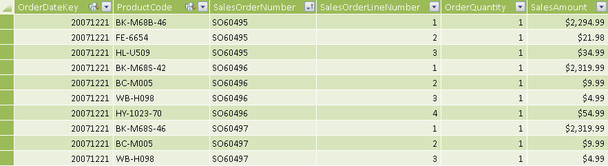
Suppose you have a Sales table containing one row for each row detail in an order. The SalesOrderNumber column identifies rows that are part of the same order, as you see in Figure 1.
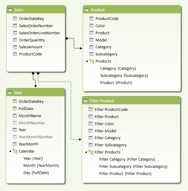
The OrderDateKey and ProductCode columns reference the Date and Product tables, respectively. The Product table contains the attributes that are the target of the analysis, such as the product name or category. You create a copy of the Product table, called Filter Product, which contains the same data and has the prefix “Filter” before all table and column names. The relationship between the Sales table and the Filter Product table is inactive, as shown in Figure 2.
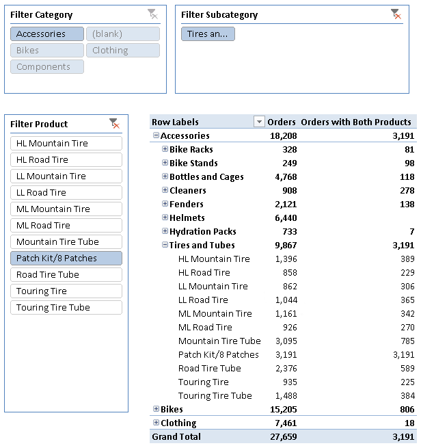
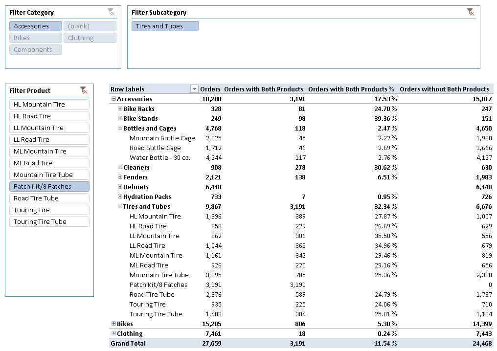
The Filter Product table enables users to specify a second product (or related attribute) as a filter in a pivot table for a measure that considers only orders that contain both products. For example, the pivot table in Figure 3 shows the number of orders of each bike accessory and, in the same row, the number of orders with that accessory plus the product filtered by the Filter Product slicer (in this case, Patch Kit/8 Patches).
The Orders measure is a simple distinct count of the SalesOrderNumber column.
[Orders] := DISTINCTCOUNT ( Sales[SalesOrderNumber] )
The Orders with Both Products measure implements a similar calculation, applying a filter that considers only the orders that also contain the product selected in the Filter Product table:
[Orders with Both Products] :=
CALCULATE (
    DISTINCTCOUNT ( Sales[SalesOrderNumber] ),
    CALCULATETABLE (
        SUMMARIZE ( Sales, Sales[SalesOrderNumber] ),
        ALL ( Product ),
        USERELATIONSHIP ( Sales[ProductCode], 'Filter Product'[Filter ProductCode] )
    )
)
This is a generic approach to basket analysis, which is useful for many different calculations, as you will see in the complete pattern.
Use Cases
You can use the Basket Analysis pattern in scenarios when you want to analyze relationships between different rows in the same table that are connected by attributes located in the same table or in lookup tables. The following is a list of some interesting use cases.
Cross-Selling
With basket analysis, you can determine which products to offer to a customer, increasing revenues and improving your relationship with the customer. For example, you can analyze the products bought together by other customers, and then offer to your customer the products bought by others with a similar purchase history.
Upselling
During the definition of an order, you can offer an upgrade, an add-on, or a more expensive item. Basket analysis helps you to identify which product mix is more successful, based on order history.
Sales Promotion
You can use purchase history to define special promotions that combine or discount certain products. Basket analysis helps you to identify a successful product mix and to evaluate the success rate of a promotion encouraging customers to buy more products in the same order.
Complete Pattern
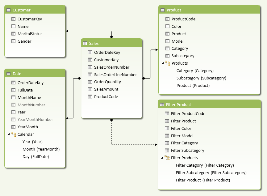
Create a data model like the one shown in Figure 4. The Filter Product table is a copy of the Product table and has the prefix “Filter” for each name (table, columns, hierarchies, and hierarchy levels). The relationship between the Sales and Filter Product tables is inactive. When doing basket analysis, users will use the Filter Product table to apply a second filter to product attributes.
The pivot table in Figure 5 shows the number of orders with different conditions depending on the selection of products made in rows and slicers.
The products hierarchy in the pivot table rows filters all the orders, and the Orders measure displays how many orders include at least one of the products selected (this is the number of orders that contain at least one of the products of the category/subcategory selected in the bold rows).
[Orders] := DISTINCTCOUNT ( Sales[SalesOrderNumber] )
The slicers around the pivot table show the selection of attributes from the Filter Product table (Filter Category, Filter Subcategory, and Filter Product). In this example, only one product is selected (Patch Kit/8 Patches). The Orders with Both Products measure shows how many orders contain at least one of the products selected in the pivot table rows and also the filtered product (Patch Kit/8 Patches) selected in the Filter Product slicer.
[Orders with Both Products] :=
CALCULATE (
    DISTINCTCOUNT ( Sales[SalesOrderNumber] ),
    CALCULATETABLE (
        SUMMARIZE ( Sales, Sales[SalesOrderNumber] ),
        ALL ( Product ),
        USERELATIONSHIP ( Sales[ProductCode], 'Filter Product'[Filter ProductCode] )
    )
)
The Orders with Both Products % measure shows the percentage of orders having both products; it is obtained by comparing the Orders with Both Products measure with the Orders measure. However, if the product selected is the same in both the Product and Filter Product tables, you hide the result returning BLANK, because it is not useful to see 100% in these cases.
[SameProductSelection] :=
IF (
    HASONEVALUE ( Product[ProductCode] )
        && HASONEVALUE ( 'Filter Product'[Filter ProductCode] ),
    IF (
        VALUES ( Product[ProductCode] )
            = VALUES ( 'Filter Product'[Filter ProductCode] ),
        TRUE
    )
)
[Orders with Both Products %] :=
IF (
    NOT ( [SameProductSelection] ),
    DIVIDE ( [Orders with Both Products], [Orders] )
)
The Orders without Both Products measure is simply the difference between Orders and Orders with Both Products measures. This number represents the number of orders containing the product selected in the pivot table, but not the product selected in the Filter Product slicer.
[Orders without Both Products] :=
[Orders] - [Orders with Both Products]
You can also create measures analyzing purchases made by each customer in different orders. The pivot table in Figure 6 shows the number of customers with different conditions depending on the selection of products in rows and slicers.
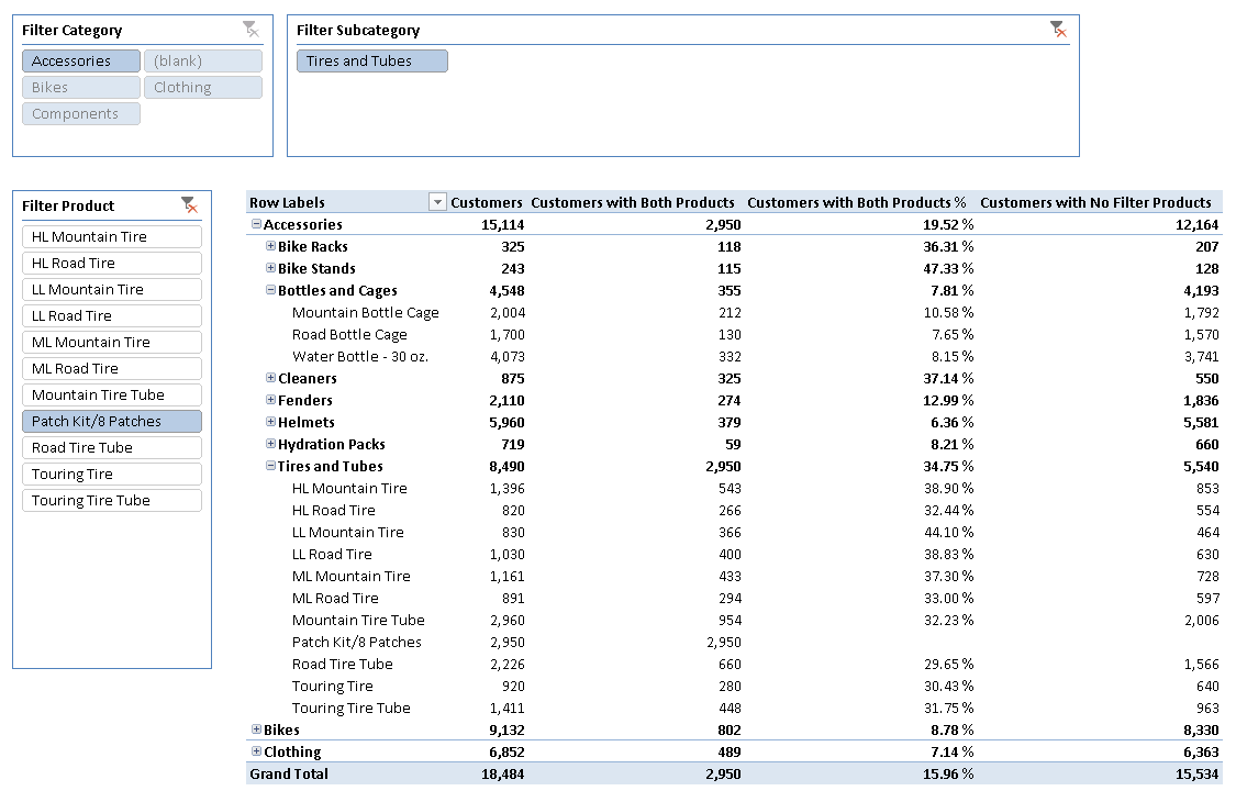
The selection in the pivot table is identical to the one used for counting orders. The measures are also similar—you just replace the distinct count calculation in the formulas, using the CustomerKey column on the Sales table.
[Customers] := DISTINCTCOUNT ( Sales[CustomerKey] )
[Customers with Both Products] :=
CALCULATE (
    DISTINCTCOUNT ( Sales[CustomerKey] ),
    CALCULATETABLE (
        SUMMARIZE ( Sales, Sales[CustomerKey] ),
        ALL ( Product ),
        USERELATIONSHIP ( Sales[ProductCode], 'Filter Product'[Filter ProductCode] )
    )
)
[Customers with Both Products %] :=
IF (
    NOT ( [SameProductSelection] ),
    DIVIDE ( [Customers with Both Products], [Customers] )
)
To count or list the number of customers who never bought the product that you want to filter for, there is a more efficient technique. Use the Customers with No Filter Products measure, as defined below.
[Customers with No Filter Products] :=
COUNTROWS (
    FILTER (
        CALCULATETABLE ( Customer, Sales ),
        ISEMPTY (
            CALCULATETABLE (
                Sales,
                ALL ( Product ),
                USERELATIONSHIP ( Sales[ProductCode], 'Filter Product'[Filter ProductCode] )
            )
        )
    )
)
You can use the result of the FILTER statement as a filter argument for a CALCULATE statement—for example, to evaluate the sales amount of the filtered selection of customers. If the ISEMPTY function is not available in your version of DAX, then use the following implementation:
[Customers with No Filter Products Classic] :=
COUNTROWS (
    FILTER (
        CALCULATETABLE ( Customer, Sales ),
        CALCULATE (
            COUNTROWS ( Sales ),
            ALL ( Product ),
            USERELATIONSHIP ( Sales[ProductCode], 'Filter Product'[Filter ProductCode] )
        )  = 0
    )
)
Important The ISEMPTY function is available only in Microsoft SQL Server 2012 Service Pack 1 Cumulative Update 4 or later versions. For this reason, ISEMPTY is available only in Power Pivot for Excel 2010 build 11.00.3368 (or later version) and SQL Server Analysis Services 2012 build 11.00.3368 (or later version). At the moment of writing, ISEMPTY is not available in any version of Excel 2013, updates of which depend on the Microsoft Office release cycle and not on SQL Server service packs.
More Pattern Examples
In this section, you will see a few examples of the Basket Analysis pattern.
Products More Likely Bought with Another Product
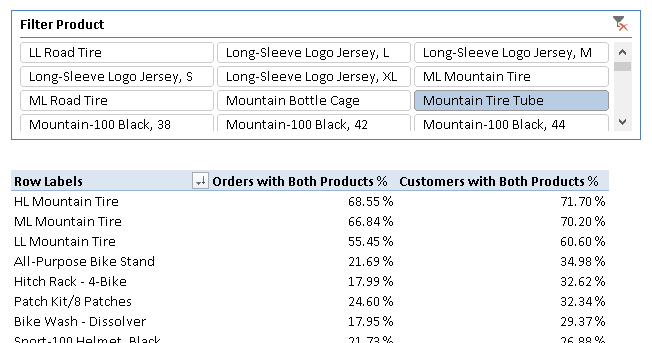
If you want to determine which products are most likely to be bought with another product, you can use a pivot table that sorts products by one of the percentage measures you have seen in the complete pattern. For example, you can use a slicer for Filter Product and place the product names in pivot table rows. You use either the Orders with Both Products % measure or the Customers with Both Products % measure to sort the products by rows, so that the first rows in the pivot table show the products that are most likely to be sold with the product selected in the slicer. The example shown in Figure 7 sorts products by the Customers with Both Products % measure in a descending way, so that you see which products are most commonly sold to customers who bought the product selected in the Filter Product slicer.
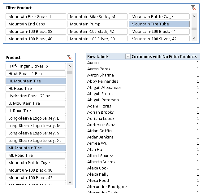
Customers Who Bought Product A and Not Product B
Once you know that certain products have a high chance to be bought together, you can obtain a list of customers who bought product A and never bought product B. You use two slicers, Product and Filter Product, selecting one or more products in each one. The pivot table has the customer names in rows. For customers who bought at least one product selected in the Product slicer but never bought any of the products selected in the Filter Product slicer, the Customers with No Filter Products measure should return 1.
The example shown in Figure 8 shows the list of customers who bought an HL Mountain Tire or an ML Mountain Tire, but never bought a Mountain Tire Tube. You may want to contact these customers and offer a Mountain Tire Tube.
Returns a blank.
BLANK ( )
Returns a table that has been filtered.
FILTER ( <Table>, <FilterExpression> )
Evaluates an expression in a context modified by filters.
CALCULATE ( <Expression> [, <Filter> [, <Filter> [, … ] ] ] )
Returns true if the specified table or table-expression is Empty.
ISEMPTY ( <Table> )
This pattern is designed for Excel 2010-2013. An alternative version for Power BI / Excel 2016-2019 is also available.
This pattern is included in the book DAX Patterns 2015.


Downloads
Download the sample files for Excel 2010-2013: