


Digital Envelope Detection: The Good, the Bad, and the Ugly
Recently I've been thinking about the process of envelope detection. Tutorial information on this topic is readily available but that information is spread out over a number of DSP textbooks and many Internet web sites. The purpose of this blog is to summarize various digital envelope detection methods in one place.
Here I focus on envelope detection as it is applied to an amplitude-fluctuating sinusoidal signal where the positive-amplitude fluctuations (the sinusoid's envelope) contain some sort of information. Let's begin by looking at the simplest envelope detection method.
Asynchronous Half-Wave Envelope Detection
Figure 1 is a digital version of a popular envelope detector used in the analog world for amplitude modulation (AM) demodulation in analog AM receivers. The job of this envelope detector is to extract (detect) the low frequency amplitude envelope signal (the dashed curve) from the incoming RF signal.
Note: Although the signal waveforms in Figure 1 appear to be continuous, keep in mind that they are indeed discrete-time numerical sequences (digital signals).
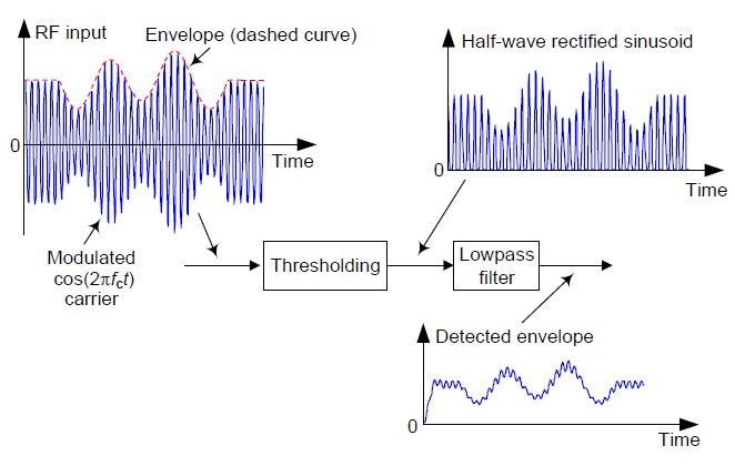
Figure 1: Asynchronous half-wave envelope detector.
Due to the harmonics (multiples of the incoming fc carrier frequency) generated by half-wave rectification in Figure 1 and possible spectral aliasing depending on the system's fs sample rate, careful spectrum analysis of the half-wave rectified sinusoid is necessary to help you determine the appropriate cutoff frequency of the digital lowpass filter. Here I used a simple third-order IIR lowpass filter to generate all of the output envelope waveforms presented in this blog.
This simple detector is called "asynchronous" because it need not generate a constant amplitude copy of the incoming RF sinusoid, as do some of the other detectors we'll be discussing.
Asynchronous Full-Wave Envelope Detection
We can reduce the high-frequency noise riding on the Figure 1 detector output by performing full-wave rectification as shown in Figure 2 [1].
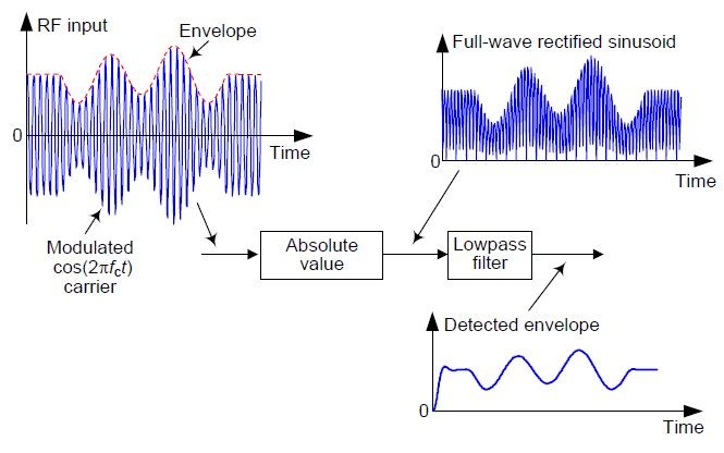
Figure 2: Asynchronous full-wave envelope detector.
Here the lowest-frequency spectral harmonic at the filter's input is 2 fc Hz. So that harmonic is more thoroughly attenuated at the Figure 2 lowpass filter output compared to the first fc Hz harmonic at the Figure 1 filter output.
Asynchronous Real Square-Law Envelope Detection
Figure 3 is a digital version of a popular square-law analog envelope detector (sometimes called a "product detector").
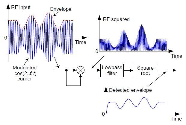
Figure 3: Asynchronous real square-law envelope detector.
Here the spectral harmonics at the filter's input are the same as those in Figure 2. References [2,3] give a mathematical description of the Figure 3 envelope detector.
Asynchronous Complex Envelope Detection
Figure 4 shows a popular digital envelope detector that uses a Hilbert transformer to compute a complex-valued version of the incoming signal. (This detector is described in more detail in Reference [4].)
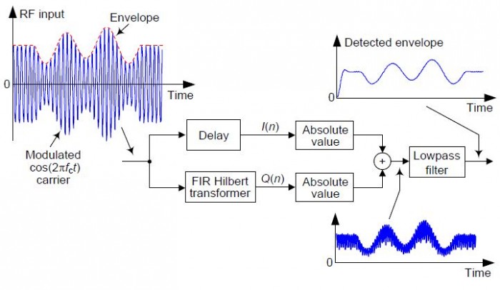
Figure 4: Asynchronous complex envelope detector.
The above Hilbert transformer need not be super high-performance, such as a wideband one whose passband extends from nearly zero Hz to nearly half the sample rate (fs/2 Hz). The transformer's passband need only be wide enough to include the spectral energy of the incoming RF signal.
Asynchronous Complex Square-Law Envelope Detection
Another digital envelope detector that uses a Hilbert transformer is shown in Figure 5. (This detector is described in more detail in References [2,3].)
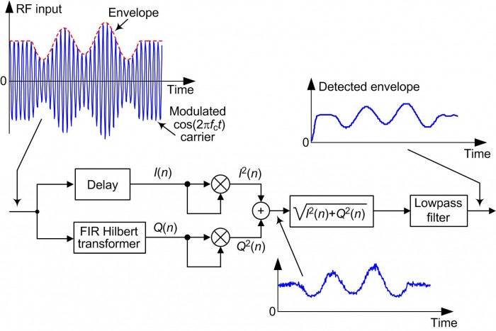
Figure 5: Asynchronous complex square-law envelope detector.
This is a most interesting envelope detector. Reference [5] touts this detector's advantage that no lowpass filtering is needed at the output of the square root operation. However, I have learned this only to be true for noise-free signals! In practical real-world applications the lowpass filter I've included in Figure 5 is necessary.
Synchronous Real Envelope Detection
Figure 6 shows an envelope detector that's called "synchronous" because the RF input signal is multiplied by a local oscillator signal whose frequency is fc Hz. (This detector is sometimes called a "coherent envelope detector.")
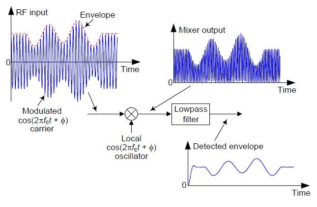
Figure 6: Synchronous Real Envelope Detector.
The complicated part of this detector is that the fc Hz carrier frequency of the received RF input signal must be regenerated (a process called "carrier recovery") within the envelope detector to provide the local oscillator's $ cos(2 \pi f_c t + \phi) $ signal. Another complication is that the local oscillator output must be in-phase with the input RF signal's sinusoid.
Reference [6] gives a detailed mathematical description of this synchronous envelope detector.
Asynchronous Complex Envelope Detection
Reference [7] proposes the Figure 7 envelope detector that compute a complex-valued version of the incoming signal.
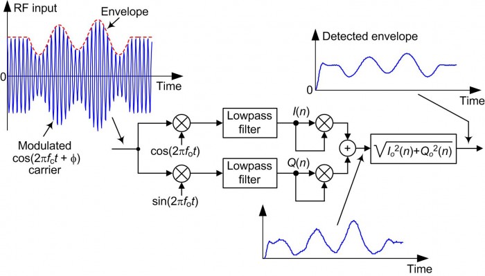
Figure 7: Asynchronous complex envelope detector.
This detector is asynchronous in operation because the local oscillators' fo frequency need not be equal to the fc frequency of the incoming modulated RF signal. An fo within 25% of fc is acceptable so long as the lowpass filters sufficiently attenuate spectral energy near |fc+fo| Hz.
Because the I(n) and Q(n) sequences are in quadrature, phase cancellation occurs in the adder such that only spectral energy in the vicinity of zero Hz appears at the adder's output. As such, this detector is very tolerant of local oscillator frequency/phase drift just so long as the local cosine/sine oscillators remain in quadrature.
Although I haven't seen it in the literature it
seemed to me that we can eliminate one of the filters in Figure 7 and implement
that envelope detector as shown in Figure 8.
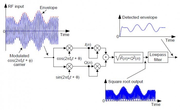
Figure 8: An alternate synchronous complex envelope detector.
Upon analysis of this Figure 8 detector I was surprised to determine that it's exactly equivalent to the Figure 2 asynchronous full-wave envelope detector! The reader can verify this by solving the following homework problem:
HOMEWORK PROBLEM FOR THE READER:
Assume an input sample to the Figure 8 detector has a value of A and the cosine oscillator's sample is $ cos(\alpha) $. What is the value of the output sample of the square root operation? Assuming the next input sample to detector has a value of -A and the cosine oscillator's next sample is $ cos(\beta) $, what is the value of the next output sample of the square root operation?
There's no reason to discuss the Figure 8 detector any further.
Detector Performance: The Good, the Bad, and the Ugly

If you'll accept the definition of "performance" to indicate a detector's output signal-to-noise ratio (SNR) for a given noisy RF input signal, you'll notice that I've presented no statistical information on the performance of the various envelope detectors here. (That was not my goal.) However, I do have a few comments regarding performance.
For applications where high accuracy is not needed, such as automatic gain control (AGC) or amplitude-shift keying (ASK) demodulation, the Figure 1 detector is attractive because it's so easy to implement. Equally easy to implement, the Figure 2 detector has been used to process medical electromyogram (EMG) signals [8].
References [9,10] show the superiority of the Figure 4 envelope detector over the Figure 2 detector in a medical ultrasound signal analysis application.
Based on my very limited modeling of the various envelope detectors, with:
• Sample rate: fs = 8000 Hz
• RF carrier frequency: 600 Hz
• Modulation: 60 Hz sine plus 30 Hz cosine wave
• Modulated RF signal SNR: +20 dB
• Lowpass filter: 3rd-order IIR (≈240 Hz cutoff frequency)
I rank the detectors' performances (from best to worst) as follows:
| Highest output SNR: | Asynch Complex (Figure 4) | |
| ↓ | Asynch Complex Square-Law (Figure 5) | |
| ↓ | Asynch Full-Wave (Figure 2) | |
| ↓ | Asynch Complex (Figure 7) | |
| ↓ | Synch Real (Figure 6) | |
| ↓ | Asynch Real Square-Law (Figure 3) | |
| Lowest output SNR: | Asynch Half-Wave (Figure 1) |
If you need an envelope detector in some real world application, I suggest you implement several of the above detectors to see which one is optimum for your signals and your fs data sample rate. To quote Forrest Gump, "And that's all I have to say about that."

References
[1] C. R. Johnson Jr., W. A. Sethares, and A. G. Klein, Software Receiver Design, Cambridge University Press, 2011, pp. 82-84.
[2] Tretter, S. A., http://www.ece.umd.edu/~tretter/commlab/c6713slides/ch5.pdf
[3] Tretter, S. A., Communication System Design Using DSP Algorithms, Springer, 2008, pp. 123-127.
[4] Lyons, R., Understanding Digital Signal Processing, 3rd Ed., Prentice Hall Publishing, 2011, pp. 786-784.
[5] Ciardullo, D.,Fast Envelope Detector, Brookhaven Nat. Lab., AGS/AD/Tech. Note No. 386, http://www.agsrhichome.bnl.gov/AGS/Accel/Reports/Tech%20Notes/TN386.pdf
[6] Abdel-Aleem, M., http://goo.gl/ErTXG9
[7] Frerking, M. E., Digital Signal Processing in Communications Systems, Chapman & Hall, 1994, pp. 235-238.
[8] Rose, W., https://www.udel.edu/biology/rosewc/kaap686/notes/EMG%20analysis.pdf
[9] Jan, J., https://goo.gl/OE8rmf
[10] Jan, J, Medical Image Processing, Reconstruction and Restoration: Concepts and Methods, CRC Press, 2005, pp. 299-300.


- Comments
- Write a Comment Select to add a comment

https://www.dsprelated.com/thread/167/envelope-detection

I'm curious about the Hilbert transformer, will have to read up on those references.
thanks!

At first I thought you were mistaken about what happens by moving the Fig. 8 square root to after the LPF. But upon modeling that scenario (with my floating point numbers), you are correct within one part in one thousand! That surprised me. Thanks for the interesting suggestion jms_nh. (Also, thanks for the beer.)
another variation of Figure 7 case is to use an NCOs (sin and cos) which has frequency different than fc so that I/Q has (fc - fnco) and (fc + fnco). LPF will eliminate (fc + fnco). rest same as Figure 7.
in short,in Figure 7, there is no need that the osc needs to be fc. they can be lower freq. however, cutoff of the LPF shall be higher than the fc-fnco.
Hello chalil. Your idea conflicts with the guidance given in the Frerking book. However, you are correct! Thanks for sharing your thoughts with us.
[-Rick-]

In Fig. 7, or any that are taking SQRT(I^2 + Q^2), how about using the approximation of P = max(abs(I),abs(Q)) + (3/8)*min(abs(I),abs(Q)) to save gates?
Hi napierm.
Yes, yes. That approximation for computing the magnitude of a complex number is what I call "alpha max plus beta min." Your suggestion is a good one! I included that approximation scheme in an IEEE article on this 'envelope detection' subject, but for some unknown reason I didn't include it here in my blog!!
Napierm, thanks for reminding all of us.

Hi Lyons,
in figure 3 , the signal is multiplied by itself . And this will double the frequency of its ! I think the recovered signal will be doubled in frequency.
Also in figure 2, the absolute value block will transform the negative half cycles to positives half cycles, I think the recovered signal will be doubled in frequency.
I tried figure 3 and 2 using Vivado IDE Simulator. As shown in the attached pictures respectively.
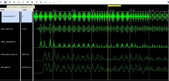
Figure 3 trial
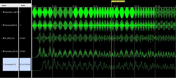
Figure 2 trial
Thanks
Hey Rick, still a great summarizing article. Also well researched with the sources for further reading.
Many thanks for this! :)
Very nice overview, thank you very much! Although I am working on an analog design, the principle is basically the same and therefore the discussion is very helpful.
However, according to my calculations and simulations, taking the square root of the signal in Figure 7 is not necessary and the result is already correct after addition. Have I missed something here?
Many Thanks,
Max
Hello HSmax.
Your comment is intriguing. It's quite possible that you detected something that *I* missed! If you performed some sort of algebraic analysis of the sum of the outputs of the two filters in my Figure 7, assuming the network's input was an unmodulated cosine wave, did you end up with an expression that looked anything like the following:
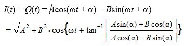
Thank you very much for your reply. I went through my analysis again and I have to apologize. I did indeed miss something (unfortunately in both the calculation and the simulation) and it is all correct as shown in Figure 7!
Hi HSmax. OK, great
Happy Easter.
Hi Rick,
thanks for sharing this convenient all-in-one-place summary.
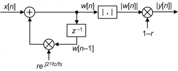
What about a solution with a quadrature first order complex recursive filter tuned to fc and followed by magnitude ? The filter equation is in this case y[n]=r*a*y[n-1]+(1-r)*x[n], where r is the feedback term defining bandwidth (e.g. 0.98), a is complex and located on the unit circle at fc, a=exp(j*2*pi*fc/fs), y is the complex quadrature output, x is real input. Then output envelope is just abs(y).
I use it for sound analysis in small-footprint embedded designs. Does it make sense to you in the context of your article ?
Regards,
Tomasz
Hello Tomasz. In your equation for 'y' you have the variable 'y' on both sides of the equation. Did you mean to write:
y[n] = r*a*y[n-1] + (1-r)*x[n]
Hello Rick, that's correct, i have edited original comment for clarity.
Hi Tomasz. OK, ...it looks like your network is an "exponential averager" (also called a "leaky integrator") whose bandpass center frequency is at fc Hz, rather than at DC (zero Hz). The block diagram is:
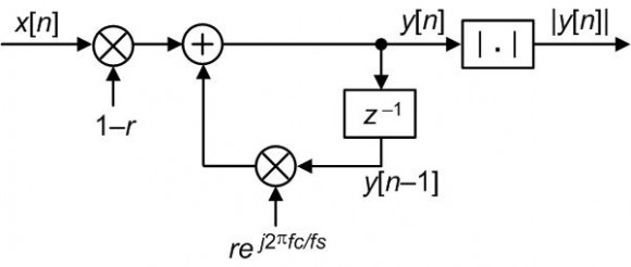
I can definitely see how your network would be useful to estimate the instantaneous envelope of a sinusoidal signal that is centered at fc Hz. If I were to use your network in practice I'd consider (think about) moving the attenuating "multiply by (1-r)" to the output as shown below:
Thanks for sharing your network with us Tomasz!!
Hi, gr8 summary.
I have a question: I have simulated a case of OOK envelope detection, in case of very bad SNR (assume negative).
What I get, is that the only scheme that works "good" is "6", all the rest, significantly boost the thermal nose and cause significant performance loss.
Do I miss anything? should I look for a mistake in my sim? or you think it is expected?
Hello guteleni.
I did not perform any sort of "low SNR performance" analysis of the above envelope detectors. So I can't say anything about their performance with very noisy input signals.
If your software simulations are performed using MATLAB code I'll be happy to have a look at your code. My e-mail address is: R.Lyons@ieee.org
To post reply to a comment, click on the 'reply' button attached to each comment. To post a new comment (not a reply to a comment) check out the 'Write a Comment' tab at the top of the comments.
Please login (on the right) if you already have an account on this platform.
Otherwise, please use this form to register (free) an join one of the largest online community for Electrical/Embedded/DSP/FPGA/ML engineers:


